Online News Analysis - Predicting Media Shares by Article Characteristics ================ Matt Kasle 10/15/2020
thursday articles
Introduction
This dataset summarizes a heterogeneous set of features about articles published by Mashable in a period of two years. The goal is to predict the number of shares in social networks (popularity).
There are 61 attributes, 58 which are predictive attributes, 2 of which are non-predictive (url and timestamp), and 1 that is the target.
The types of veriables include the number of words in the article, the number of words in the title, the positivity and sentimentality of the article, the article’s subject, the number of keywords used, and much more.
The objective of this project is to predict the number of social media shares using two different tree-based algorithms. The first algorithm will be a non-ensemble regression tree, and the second algorithm will be a boosted trees algorithm, which is a state-of-the-art classification technique.
The other objective of this project is to create an automated report that outputs the classification analysis for each articles published on each weekday.
The required packages to run this analysis are tidyverse, caret, tree, and patchwork.
Data
First, we need to read in the data and set up the subsetting of the data into a single weekday. Then, we’ll split the data set to a training and test set for training and evaluating the classificaiton models. A 70/30 train-test split will be used.
set.seed(1)
library(tidyverse)
library(caret)
library(tree)

news <- read_csv("OnlineNewsPopularity.csv")
varDayOfWeek <- parse(text=paste0("weekday_is_", params$day_of_week))
news <- news %>% filter(eval(varDayOfWeek) == 1)

news <- news %>% select(-url, -timedelta, -weekday_is_monday, -weekday_is_tuesday, -weekday_is_wednesday,
                        -weekday_is_thursday,-weekday_is_friday,
                        -weekday_is_saturday, -weekday_is_sunday, -is_weekend)

newsIndex <- createDataPartition(news$shares, p = 0.3, list = FALSE)
newsTrain <- news[newsIndex, ]
newsTest <- news[-newsIndex, ]
Summarizations
Below are summary statistics of the online news data set, such as the number of observations in the train set, a numerical summary of the response variable (number of social media shares), a distribution of the response, and relationships between the response and interesting variables in the dataset.
Number of rows in training set:
nrow(newsTrain)
## [1] 2183
Summary of response variable:
summary(newsTrain$shares)
##     Min.  1st Qu.   Median     Mean  3rd Qu.     Max.
##     22.0    901.5   1400.0   2953.3   2600.0 227300.0
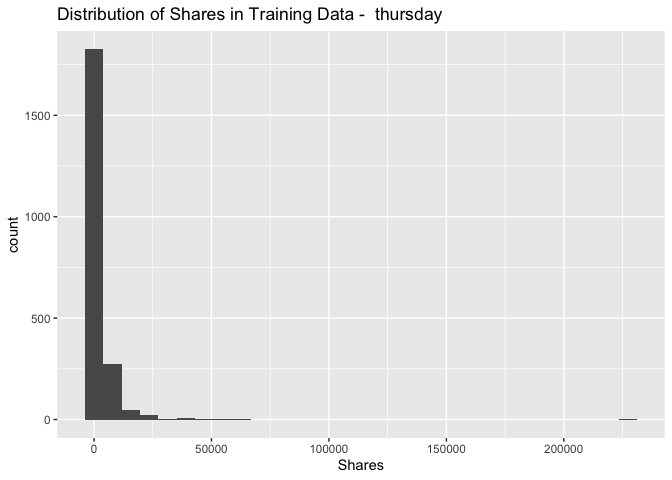
It is important to make note of the minimum and maximum of the response variable, as well as the median and quartiles. For future analysis, it may be best to remove outliers.
Distribution of response variable:
ggplot(data = newsTrain, aes(x = shares)) +
  geom_histogram() + xlab("Shares") + ggtitle(paste("Distribution of Shares in Training Data - ",
                                                    params$day_of_week))
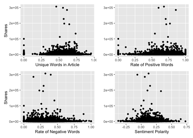
Below is a plot of four interesting variables to the response variable, shares. We want to see if there are any intersting patterns here.
library(patchwork)
par(mfrow=c(2,2))
plot1 <- ggplot(data=news, aes(x = news$n_unique_tokens, y = shares)) + geom_point(stat = "identity") +
    labs(x="Unique Words in Article", y="Shares")

plot2 <- ggplot(data=news, aes(x = news$rate_positive_words, y = shares)) + geom_point(stat = "identity") +
    labs(x="Rate of Positive Words", y="")

plot3 <- ggplot(data=news, aes(x = news$rate_negative_words, y = shares)) + geom_point(stat = "identity") +
    labs(x="Rate of Negative Words", y="Shares")

plot4 <- ggplot(data=news, aes(x = news$global_sentiment_polarity, y = shares)) + geom_point(stat = "identity") +
    labs(x="Sentiment Polarity", y="")

plot1 + plot2 + plot3 + plot4
## Warning: Use of `news$n_unique_tokens` is discouraged. Use `n_unique_tokens` instead.

## Warning: Use of `news$rate_positive_words` is discouraged. Use `rate_positive_words` instead.

## Warning: Use of `news$rate_negative_words` is discouraged. Use `rate_negative_words` instead.

## Warning: Use of `news$global_sentiment_polarity` is discouraged. Use `global_sentiment_polarity` instead.
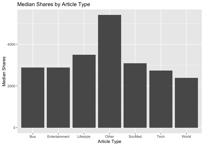
There are six different article subjects. It would be interesting to know if some subjects are more popular than others, so we can plot the median shares by the different article types.
news['article_type'] <- ifelse(news$data_channel_is_lifestyle == 1, "Lifestyle",
       ifelse(news$data_channel_is_entertainment == 1, "Entertainment",
       ifelse(news$data_channel_is_world == 1, "World",
       ifelse(news$data_channel_is_bus == 1, "Bus",
       ifelse(news$data_channel_is_socmed == 1, "SocMed",
       ifelse(news$data_channel_is_tech == 1, "Tech","Other"))))))

ggplot(data=news, aes(x = article_type, y = shares)) + geom_bar(stat = "summary", fun.y = "median") +
    labs(x="Article Type", y="Median Shares", title="Median Shares by Article Type")
## Warning: Ignoring unknown parameters: fun.y

## No summary function supplied, defaulting to `mean_se()`
# drop column used for plotting
news <- news %>% select(-article_type)
Modeling
There should be text describing the type of model you are fitting, your fitting process, and the final chosen model (this last part is to be automated so I don’t expect you to explicitly interpret that model, but you should be able to display something about the final model chosen on the training data).
Regression Tree Model
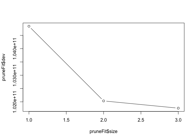
The first model fit to the data will be a regression tree. We’ll use leave-one-out cross-validation to determine the optimal size of the model, as defined by number of splits. By plotting the fitted tree, we can see the deviance by tree size (larger deviance means a better fit).
treeFit <- tree(shares ~ ., data = newsTrain)
summary(treeFit)
##
## Regression tree:
## tree(formula = shares ~ ., data = newsTrain)
## Variables actually used in tree construction:
## [1] "kw_avg_avg" "num_hrefs"
## Number of terminal nodes:  3
## Residual mean deviance:  45320000 = 9.881e+10 / 2180
## Distribution of residuals:
##     Min.  1st Qu.   Median     Mean  3rd Qu.     Max.
## -15110.0  -1766.0  -1341.0      0.0   -240.8 224800.0
pruneFit <- cv.tree(treeFit,
                  K=nrow(newsTrain)-1
                  )


pruneFitFinal <- prune.tree(treeFit, best = pruneFit$size[1])

plot(pruneFit$size ,pruneFit$dev ,type="b")
Boosted tree model
Next, we’ll fit a boosted regression tree. The boosted tree algorithm has a few hyperparameters, and we’ll use repeated 10-fold cross-validation to determine the optimal hyperparameter values. The hyperparameters of the optimal boosted tree is printed below, as well a summary of each fitted model.
fitControl <- trainControl(## 10-fold CV
                           method = "repeatedcv",
                           number = 10,
                           ## repeated ten times
                           repeats = 5
                           )

boostedFit <- train(shares ~ ., data = newsTrain,
                 method = "gbm",
                 trControl = fitControl,
                 verbose = FALSE
                 )

boostedFit$bestTune
##   n.trees interaction.depth shrinkage n.minobsinnode
## 1      50                 1       0.1             10
boostedFit$results
##   shrinkage interaction.depth n.minobsinnode n.trees     RMSE   Rsquared      MAE   RMSESD RsquaredSD    MAESD
## 1       0.1                 1             10      50 5819.285 0.03995600 2506.175 3536.858 0.03456849 365.8769
## 4       0.1                 2             10      50 6005.761 0.02323220 2573.457 3478.829 0.02298231 370.3773
## 7       0.1                 3             10      50 6016.262 0.02819922 2600.250 3466.042 0.02829338 359.0629
## 2       0.1                 1             10     100 5844.459 0.04238553 2528.208 3533.218 0.03730936 379.1860
## 5       0.1                 2             10     100 6151.887 0.02110848 2679.940 3438.671 0.02428009 366.0115
## 8       0.1                 3             10     100 6182.216 0.02420803 2733.599 3416.553 0.02634264 352.4273
## 3       0.1                 1             10     150 5848.139 0.04468921 2537.955 3529.133 0.03863956 375.5992
## 6       0.1                 2             10     150 6214.168 0.02065998 2753.700 3419.594 0.02516954 359.3457
## 9       0.1                 3             10     150 6296.936 0.02211659 2837.559 3380.756 0.02444534 338.3367
Linear regression model
Next, we’ll fit a multiple linear regression model on train data. Summary of the model is printed below.
linearfit<-lm(shares~.,data=newsTrain)
summary(linearfit)
##
## Call:
## lm(formula = shares ~ ., data = newsTrain)
##
## Residuals:
##    Min     1Q Median     3Q    Max
##  -9605  -2072   -901    341 218909
##
## Coefficients: (2 not defined because of singularities)
##                                 Estimate Std. Error t value Pr(>|t|)
## (Intercept)                    3.140e+03  2.273e+03   1.382  0.16723
## n_tokens_title                 1.115e+02  7.118e+01   1.566  0.11739
## n_tokens_content              -4.133e-01  6.267e-01  -0.659  0.50969
## n_unique_tokens                6.147e+02  4.958e+03   0.124  0.90134
## n_non_stop_words              -4.340e+03  4.174e+03  -1.040  0.29857
## n_non_stop_unique_tokens      -4.447e+02  4.130e+03  -0.108  0.91428
## num_hrefs                      5.697e+01  1.896e+01   3.005  0.00269 **
## num_self_hrefs                 6.094e+00  4.714e+01   0.129  0.89715
## num_imgs                      -1.644e+01  2.419e+01  -0.680  0.49667
## num_videos                    -1.729e+01  5.032e+01  -0.344  0.73111
## average_token_length          -1.346e+02  6.152e+02  -0.219  0.82688
## num_keywords                  -2.594e+02  9.308e+01  -2.787  0.00536 **
## data_channel_is_lifestyle     -1.696e+02  1.008e+03  -0.168  0.86642
## data_channel_is_entertainment -1.786e+03  6.825e+02  -2.617  0.00893 **
## data_channel_is_bus           -1.280e+03  9.544e+02  -1.341  0.18018
## data_channel_is_socmed        -1.496e+03  8.812e+02  -1.697  0.08975 .
## data_channel_is_tech          -7.808e+02  9.303e+02  -0.839  0.40138
## data_channel_is_world         -5.451e+02  9.388e+02  -0.581  0.56153
## kw_min_min                     9.052e+00  4.311e+00   2.100  0.03589 *
## kw_max_min                    -7.642e-02  1.882e-01  -0.406  0.68467
## kw_avg_min                     5.136e-01  1.238e+00   0.415  0.67830
## kw_min_max                     3.129e-03  2.484e-03   1.260  0.20780
## kw_max_max                     2.551e-03  1.498e-03   1.703  0.08871 .
## kw_avg_max                    -4.905e-03  2.092e-03  -2.345  0.01912 *
## kw_min_avg                    -2.836e-01  2.018e-01  -1.406  0.15998
## kw_max_avg                    -1.135e-01  8.572e-02  -1.324  0.18570
## kw_avg_avg                     1.056e+00  4.116e-01   2.565  0.01037 *
## self_reference_min_shares     -4.211e-02  2.828e-02  -1.489  0.13660
## self_reference_max_shares     -2.589e-02  1.855e-02  -1.396  0.16283
## self_reference_avg_sharess     7.278e-02  4.497e-02   1.618  0.10573
## LDA_00                        -8.644e+02  1.138e+03  -0.760  0.44757
## LDA_01                        -7.880e+02  1.306e+03  -0.603  0.54634
## LDA_02                        -1.638e+03  1.128e+03  -1.453  0.14650
## LDA_03                        -8.088e+02  1.229e+03  -0.658  0.51057
## LDA_04                                NA         NA      NA       NA
## global_subjectivity            3.976e+03  2.139e+03   1.859  0.06314 .
## global_sentiment_polarity     -1.312e+03  3.968e+03  -0.331  0.74096
## global_rate_positive_words     9.802e+03  1.761e+04   0.557  0.57787
## global_rate_negative_words     2.584e+03  3.547e+04   0.073  0.94193
## rate_positive_words            1.464e+02  2.865e+03   0.051  0.95924
## rate_negative_words                   NA         NA      NA       NA
## avg_positive_polarity          3.200e+03  3.388e+03   0.944  0.34511
## min_positive_polarity         -2.312e+03  2.774e+03  -0.833  0.40477
## max_positive_polarity         -1.078e+02  1.086e+03  -0.099  0.92098
## avg_negative_polarity          1.297e+03  3.245e+03   0.400  0.68936
## min_negative_polarity         -1.603e+03  1.193e+03  -1.344  0.17905
## max_negative_polarity          9.321e+02  2.668e+03   0.349  0.72683
## title_subjectivity            -7.284e+02  6.692e+02  -1.089  0.27647
## title_sentiment_polarity      -1.015e+03  6.477e+02  -1.567  0.11715
## abs_title_subjectivity         6.564e+01  9.315e+02   0.070  0.94383
## abs_title_sentiment_polarity   1.557e+03  1.019e+03   1.527  0.12684
## ---
## Signif. codes:  0 '***' 0.001 '**' 0.01 '*' 0.05 '.' 0.1 ' ' 1
##
## Residual standard error: 6708 on 2134 degrees of freedom
## Multiple R-squared:  0.05389,    Adjusted R-squared:  0.03261
## F-statistic: 2.532 on 48 and 2134 DF,  p-value: 5.03e-08
Model Evaluations
Finally, we’ll evaluate the performance of each model by seeking the lowest root mean squared error of its predictions on the test dataset when compared to the actual values in the dataset. This should be a good approximation of the model’s performance on unseen data.
Regression Tree
Below is the RMSE of the optimal (non-ensemble) regression tree:
treePred <- predict(pruneFitFinal, newdata = dplyr::select(newsTest, -shares))
sqrt(mean((treePred-newsTest$shares)^2))
## [1] 10320.2
Boosted Trees
Below is the RMSE of the optimal boosted regression tree:
boostedTreePred <- predict(boostedFit, newdata = dplyr::select(newsTest, -shares))
sqrt(mean((boostedTreePred-newsTest$shares)^2))
## [1] 10285.08
linear regression
Below is the RMSE of the multiple linear model:
linearPred<-predict(linearfit, newdata=dplyr::select(newsTest, -shares))
sqrt(mean((linearPred-newsTest$shares)^2))
## [1] 10329.17