Online News Analysis - Predicting Media Shares by Article Characteristics ================ Matt Kasle 10/15/2020
sunday articles
Introduction
This dataset summarizes a heterogeneous set of features about articles published by Mashable in a period of two years. The goal is to predict the number of shares in social networks (popularity).
There are 61 attributes, 58 which are predictive attributes, 2 of which are non-predictive (url and timestamp), and 1 that is the target.
The types of veriables include the number of words in the article, the number of words in the title, the positivity and sentimentality of the article, the article’s subject, the number of keywords used, and much more.
The objective of this project is to predict the number of social media shares using two different tree-based algorithms. The first algorithm will be a non-ensemble regression tree, and the second algorithm will be a boosted trees algorithm, which is a state-of-the-art classification technique.
The other objective of this project is to create an automated report that outputs the classification analysis for each articles published on each weekday.
The required packages to run this analysis are tidyverse, caret, tree, and patchwork.
Data
First, we need to read in the data and set up the subsetting of the data into a single weekday. Then, we’ll split the data set to a training and test set for training and evaluating the classificaiton models. A 70/30 train-test split will be used.
set.seed(1)
library(tidyverse)
library(caret)
library(tree)

news <- read_csv("OnlineNewsPopularity.csv")
varDayOfWeek <- parse(text=paste0("weekday_is_", params$day_of_week))
news <- news %>% filter(eval(varDayOfWeek) == 1)

news <- news %>% select(-url, -timedelta, -weekday_is_monday, -weekday_is_tuesday, -weekday_is_wednesday,
                        -weekday_is_thursday,-weekday_is_friday,
                        -weekday_is_saturday, -weekday_is_sunday, -is_weekend)

newsIndex <- createDataPartition(news$shares, p = 0.3, list = FALSE)
newsTrain <- news[newsIndex, ]
newsTest <- news[-newsIndex, ]
Summarizations
Below are summary statistics of the online news data set, such as the number of observations in the train set, a numerical summary of the response variable (number of social media shares), a distribution of the response, and relationships between the response and interesting variables in the dataset.
Number of rows in training set:
nrow(newsTrain)
## [1] 824
Summary of response variable:
summary(newsTrain$shares)
##    Min. 1st Qu.  Median    Mean 3rd Qu.    Max.
##      91    1200    1900    3924    3700   64500
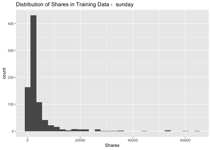
It is important to make note of the minimum and maximum of the response variable, as well as the median and quartiles. For future analysis, it may be best to remove outliers.
Distribution of response variable:
ggplot(data = newsTrain, aes(x = shares)) +
  geom_histogram() + xlab("Shares") + ggtitle(paste("Distribution of Shares in Training Data - ",
                                                    params$day_of_week))
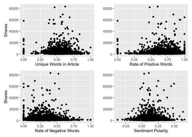
Below is a plot of four interesting variables to the response variable, shares. We want to see if there are any intersting patterns here.
library(patchwork)
par(mfrow=c(2,2))
plot1 <- ggplot(data=news, aes(x = news$n_unique_tokens, y = shares)) + geom_point(stat = "identity") +
    labs(x="Unique Words in Article", y="Shares")

plot2 <- ggplot(data=news, aes(x = news$rate_positive_words, y = shares)) + geom_point(stat = "identity") +
    labs(x="Rate of Positive Words", y="")

plot3 <- ggplot(data=news, aes(x = news$rate_negative_words, y = shares)) + geom_point(stat = "identity") +
    labs(x="Rate of Negative Words", y="Shares")

plot4 <- ggplot(data=news, aes(x = news$global_sentiment_polarity, y = shares)) + geom_point(stat = "identity") +
    labs(x="Sentiment Polarity", y="")

plot1 + plot2 + plot3 + plot4
## Warning: Use of `news$n_unique_tokens` is discouraged. Use `n_unique_tokens` instead.

## Warning: Use of `news$rate_positive_words` is discouraged. Use `rate_positive_words` instead.

## Warning: Use of `news$rate_negative_words` is discouraged. Use `rate_negative_words` instead.

## Warning: Use of `news$global_sentiment_polarity` is discouraged. Use `global_sentiment_polarity` instead.
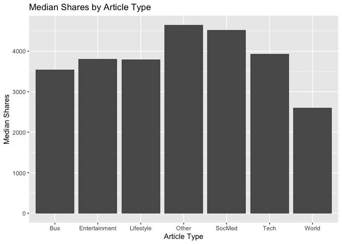
There are six different article subjects. It would be interesting to know if some subjects are more popular than others, so we can plot the median shares by the different article types.
news['article_type'] <- ifelse(news$data_channel_is_lifestyle == 1, "Lifestyle",
       ifelse(news$data_channel_is_entertainment == 1, "Entertainment",
       ifelse(news$data_channel_is_world == 1, "World",
       ifelse(news$data_channel_is_bus == 1, "Bus",
       ifelse(news$data_channel_is_socmed == 1, "SocMed",
       ifelse(news$data_channel_is_tech == 1, "Tech","Other"))))))

ggplot(data=news, aes(x = article_type, y = shares)) + geom_bar(stat = "summary", fun.y = "median") +
    labs(x="Article Type", y="Median Shares", title="Median Shares by Article Type")
## Warning: Ignoring unknown parameters: fun.y

## No summary function supplied, defaulting to `mean_se()`
# drop column used for plotting
news <- news %>% select(-article_type)
Modeling
There should be text describing the type of model you are fitting, your fitting process, and the final chosen model (this last part is to be automated so I don’t expect you to explicitly interpret that model, but you should be able to display something about the final model chosen on the training data).
Regression Tree Model
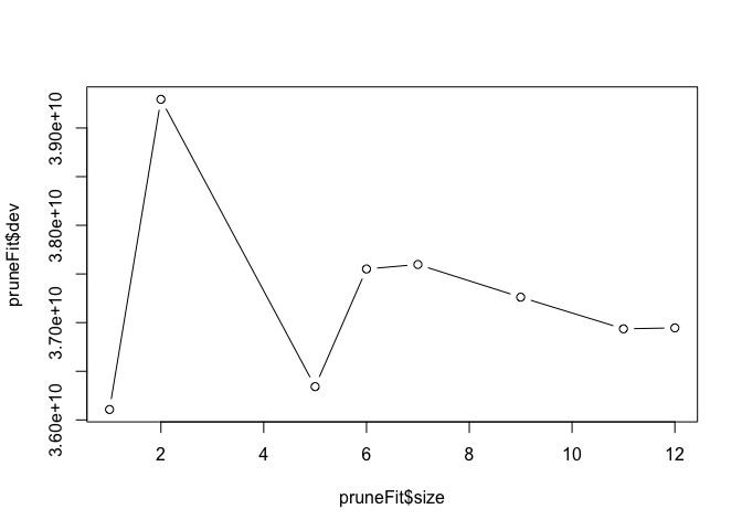
The first model fit to the data will be a regression tree. We’ll use leave-one-out cross-validation to determine the optimal size of the model, as defined by number of splits. By plotting the fitted tree, we can see the deviance by tree size (larger deviance means a better fit).
treeFit <- tree(shares ~ ., data = newsTrain)
summary(treeFit)
##
## Regression tree:
## tree(formula = shares ~ ., data = newsTrain)
## Variables actually used in tree construction:
##  [1] "self_reference_min_shares" "kw_min_avg"                "avg_positive_polarity"     "kw_max_avg"
##  [5] "rate_negative_words"       "LDA_03"                    "LDA_04"                    "avg_negative_polarity"
##  [9] "kw_max_min"                "kw_avg_max"
## Number of terminal nodes:  12
## Residual mean deviance:  28620000 = 2.324e+10 / 812
## Distribution of residuals:
##    Min. 1st Qu.  Median    Mean 3rd Qu.    Max.
##  -22120   -2043    -936       0     264   44880
pruneFit <- cv.tree(treeFit,
                  K=nrow(newsTrain)-1
                  )


pruneFitFinal <- prune.tree(treeFit, best = pruneFit$size[1])

plot(pruneFit$size ,pruneFit$dev ,type="b")
Boosted tree model
Next, we’ll fit a boosted regression tree. The boosted tree algorithm has a few hyperparameters, and we’ll use repeated 10-fold cross-validation to determine the optimal hyperparameter values. The hyperparameters of the optimal boosted tree is printed below, as well a summary of each fitted model.
fitControl <- trainControl(## 10-fold CV
                           method = "repeatedcv",
                           number = 10,
                           ## repeated ten times
                           repeats = 5
                           )

boostedFit <- train(shares ~ ., data = newsTrain,
                 method = "gbm",
                 trControl = fitControl,
                 verbose = FALSE
                 )

boostedFit$bestTune
##   n.trees interaction.depth shrinkage n.minobsinnode
## 1      50                 1       0.1             10
boostedFit$results
##   shrinkage interaction.depth n.minobsinnode n.trees     RMSE   Rsquared      MAE   RMSESD RsquaredSD    MAESD
## 1       0.1                 1             10      50 6266.247 0.04460433 3333.600 1584.036 0.06655842 457.5225
## 4       0.1                 2             10      50 6274.723 0.05515840 3354.224 1504.153 0.09106202 424.3293
## 7       0.1                 3             10      50 6308.617 0.04625092 3381.136 1509.425 0.07336252 432.3686
## 2       0.1                 1             10     100 6339.620 0.04363465 3416.257 1556.192 0.06570047 455.4007
## 5       0.1                 2             10     100 6409.929 0.04772949 3460.574 1470.997 0.07419314 451.6148
## 8       0.1                 3             10     100 6429.420 0.04357450 3501.758 1454.633 0.05691881 424.5925
## 3       0.1                 1             10     150 6410.235 0.03856114 3480.430 1526.450 0.05542399 461.7136
## 6       0.1                 2             10     150 6473.355 0.04487700 3547.440 1459.391 0.06934638 458.0592
## 9       0.1                 3             10     150 6518.688 0.04037359 3592.120 1415.080 0.05214736 430.1174
Linear regression model
Next, we’ll fit a multiple linear regression model on train data. Summary of the model is printed below.
linearfit<-lm(shares~.,data=newsTrain)
summary(linearfit)
##
## Call:
## lm(formula = shares ~ ., data = newsTrain)
##
## Residuals:
##    Min     1Q Median     3Q    Max
## -17941  -2431   -997    461  51619
##
## Coefficients: (2 not defined because of singularities)
##                                 Estimate Std. Error t value Pr(>|t|)
## (Intercept)                   -4.345e+03  3.191e+03  -1.362  0.17372
## n_tokens_title                 5.818e+01  1.103e+02   0.528  0.59794
## n_tokens_content              -3.930e-01  6.883e-01  -0.571  0.56818
## n_unique_tokens               -3.561e+03  6.688e+03  -0.532  0.59455
## n_non_stop_words              -6.955e+03  6.091e+03  -1.142  0.25383
## n_non_stop_unique_tokens       3.386e+03  5.717e+03   0.592  0.55391
## num_hrefs                      1.188e+01  1.997e+01   0.595  0.55208
## num_self_hrefs                -4.145e+00  5.345e+01  -0.078  0.93821
## num_imgs                       4.612e+00  3.066e+01   0.150  0.88046
## num_videos                     2.334e+01  6.187e+01   0.377  0.70614
## average_token_length           7.107e+02  8.576e+02   0.829  0.40755
## num_keywords                   3.486e+02  1.396e+02   2.496  0.01275 *
## data_channel_is_lifestyle      2.768e+02  1.236e+03   0.224  0.82284
## data_channel_is_entertainment  2.244e+03  8.706e+02   2.578  0.01012 *
## data_channel_is_bus            2.719e+03  1.524e+03   1.785  0.07471 .
## data_channel_is_socmed         4.009e+03  1.345e+03   2.982  0.00296 **
## data_channel_is_tech           2.238e+03  1.350e+03   1.658  0.09779 .
## data_channel_is_world          1.175e+03  1.355e+03   0.867  0.38597
## kw_min_min                     8.025e-01  5.923e+00   0.135  0.89226
## kw_max_min                     1.311e-01  3.499e-01   0.375  0.70807
## kw_avg_min                     1.105e-01  1.088e+00   0.102  0.91913
## kw_min_max                    -2.002e-03  6.951e-03  -0.288  0.77341
## kw_max_max                    -2.070e-03  2.190e-03  -0.945  0.34482
## kw_avg_max                     1.691e-03  3.379e-03   0.500  0.61690
## kw_min_avg                     5.738e-02  2.840e-01   0.202  0.83996
## kw_max_avg                    -2.218e-01  9.547e-02  -2.324  0.02039 *
## kw_avg_avg                     1.491e+00  5.508e-01   2.707  0.00693 **
## self_reference_min_shares      2.032e-01  3.656e-02   5.558 3.76e-08 ***
## self_reference_max_shares      1.264e-03  8.976e-03   0.141  0.88808
## self_reference_avg_sharess    -1.786e-02  3.638e-02  -0.491  0.62371
## LDA_00                        -1.872e+03  1.950e+03  -0.960  0.33736
## LDA_01                         2.364e+02  1.824e+03   0.130  0.89694
## LDA_02                         2.829e+01  1.771e+03   0.016  0.98726
## LDA_03                         9.887e+02  1.707e+03   0.579  0.56257
## LDA_04                                NA         NA      NA       NA
## global_subjectivity           -3.874e+03  3.114e+03  -1.244  0.21380
## global_sentiment_polarity      3.991e+03  5.722e+03   0.697  0.48577
## global_rate_positive_words    -1.492e+04  2.478e+04  -0.602  0.54737
## global_rate_negative_words     2.276e+04  5.145e+04   0.442  0.65834
## rate_positive_words            5.730e+03  4.257e+03   1.346  0.17874
## rate_negative_words                   NA         NA      NA       NA
## avg_positive_polarity          1.787e+03  4.831e+03   0.370  0.71158
## min_positive_polarity          2.139e+02  4.389e+03   0.049  0.96114
## max_positive_polarity         -1.761e+03  1.634e+03  -1.078  0.28142
## avg_negative_polarity         -1.320e+03  4.636e+03  -0.285  0.77602
## min_negative_polarity         -8.273e+02  1.670e+03  -0.495  0.62045
## max_negative_polarity          3.117e+03  3.898e+03   0.800  0.42407
## title_subjectivity             1.303e+03  1.047e+03   1.245  0.21337
## title_sentiment_polarity       7.666e-01  8.427e+02   0.001  0.99927
## abs_title_subjectivity         2.361e+03  1.274e+03   1.853  0.06428 .
## abs_title_sentiment_polarity   5.912e+01  1.405e+03   0.042  0.96644
## ---
## Signif. codes:  0 '***' 0.001 '**' 0.01 '*' 0.05 '.' 0.1 ' ' 1
##
## Residual standard error: 5984 on 775 degrees of freedom
## Multiple R-squared:  0.1888, Adjusted R-squared:  0.1386
## F-statistic: 3.758 on 48 and 775 DF,  p-value: 4.806e-15
Model Evaluations
Finally, we’ll evaluate the performance of each model by seeking the lowest root mean squared error of its predictions on the test dataset when compared to the actual values in the dataset. This should be a good approximation of the model’s performance on unseen data.
Regression Tree
Below is the RMSE of the optimal (non-ensemble) regression tree:
treePred <- predict(pruneFitFinal, newdata = dplyr::select(newsTest, -shares))
sqrt(mean((treePred-newsTest$shares)^2))
## [1] 7099.371
Boosted Trees
Below is the RMSE of the optimal boosted regression tree:
boostedTreePred <- predict(boostedFit, newdata = dplyr::select(newsTest, -shares))
sqrt(mean((boostedTreePred-newsTest$shares)^2))
## [1] 6314.956
linear regression
Below is the RMSE of the multiple linear model:
linearPred<-predict(linearfit, newdata=dplyr::select(newsTest, -shares))
sqrt(mean((linearPred-newsTest$shares)^2))
## [1] 8835.276