Online News Analysis - Predicting Media Shares by Article Characteristics ================ Matt Kasle 10/15/2020
monday articles
Introduction
This dataset summarizes a heterogeneous set of features about articles published by Mashable in a period of two years. The goal is to predict the number of shares in social networks (popularity).
There are 61 attributes, 58 which are predictive attributes, 2 of which are non-predictive (url and timestamp), and 1 that is the target.
The types of veriables include the number of words in the article, the number of words in the title, the positivity and sentimentality of the article, the article’s subject, the number of keywords used, and much more.
The objective of this project is to predict the number of social media shares using two different tree-based algorithms. The first algorithm will be a non-ensemble regression tree, and the second algorithm will be a boosted trees algorithm, which is a state-of-the-art classification technique.
The other objective of this project is to create an automated report that outputs the classification analysis for each articles published on each weekday.
The required packages to run this analysis are tidyverse, caret, tree, and patchwork.
Data
First, we need to read in the data and set up the subsetting of the data into a single weekday. Then, we’ll split the data set to a training and test set for training and evaluating the classificaiton models. A 70/30 train-test split will be used.
set.seed(1)
library(tidyverse)
library(caret)
library(tree)

news <- read_csv("OnlineNewsPopularity.csv")
varDayOfWeek <- parse(text=paste0("weekday_is_", params$day_of_week))
news <- news %>% filter(eval(varDayOfWeek) == 1)

news <- news %>% select(-url, -timedelta, -weekday_is_monday, -weekday_is_tuesday, -weekday_is_wednesday,
                        -weekday_is_thursday,-weekday_is_friday,
                        -weekday_is_saturday, -weekday_is_sunday, -is_weekend)

newsIndex <- createDataPartition(news$shares, p = 0.3, list = FALSE)
newsTrain <- news[newsIndex, ]
## Warning: The `i` argument of ``[`()` can't be a matrix as of tibble 3.0.0.
## Convert to a vector.
## This warning is displayed once every 8 hours.
## Call `lifecycle::last_warnings()` to see where this warning was generated.
newsTest <- news[-newsIndex, ]
Summarizations
Below are summary statistics of the online news data set, such as the number of observations in the train set, a numerical summary of the response variable (number of social media shares), a distribution of the response, and relationships between the response and interesting variables in the dataset.
Number of rows in training set:
nrow(newsTrain)
## [1] 2000
Summary of response variable:
summary(newsTrain$shares)
##    Min. 1st Qu.  Median    Mean 3rd Qu.    Max.
##       4     919    1400    3742    2700  690400
It is important to make note of the minimum and maximum of the response variable, as well as the median and quartiles. For future analysis, it may be best to remove outliers.
Distribution of response variable:
ggplot(data = newsTrain, aes(x = shares)) +
  geom_histogram() + xlab("Shares") + ggtitle(paste("Distribution of Shares in Training Data - ",
                                                    params$day_of_week))

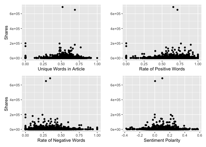
Below is a plot of four interesting variables to the response variable, shares. We want to see if there are any intersting patterns here.
library(patchwork)
## Warning: package 'patchwork' was built under R version 3.6.2
par(mfrow=c(2,2))
plot1 <- ggplot(data=news, aes(x = news$n_unique_tokens, y = shares)) + geom_point(stat = "identity") +
    labs(x="Unique Words in Article", y="Shares")

plot2 <- ggplot(data=news, aes(x = news$rate_positive_words, y = shares)) + geom_point(stat = "identity") +
    labs(x="Rate of Positive Words", y="")

plot3 <- ggplot(data=news, aes(x = news$rate_negative_words, y = shares)) + geom_point(stat = "identity") +
    labs(x="Rate of Negative Words", y="Shares")

plot4 <- ggplot(data=news, aes(x = news$global_sentiment_polarity, y = shares)) + geom_point(stat = "identity") +
    labs(x="Sentiment Polarity", y="")

plot1 + plot2 + plot3 + plot4
## Warning: Use of `news$n_unique_tokens` is discouraged. Use `n_unique_tokens` instead.

## Warning: Use of `news$rate_positive_words` is discouraged. Use `rate_positive_words` instead.

## Warning: Use of `news$rate_negative_words` is discouraged. Use `rate_negative_words` instead.

## Warning: Use of `news$global_sentiment_polarity` is discouraged. Use `global_sentiment_polarity` instead.
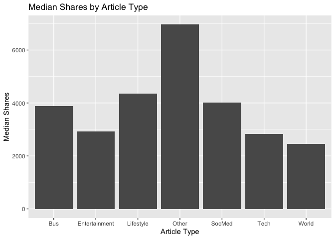
There are six different article subjects. It would be interesting to know if some subjects are more popular than others, so we can plot the median shares by the different article types.
news['article_type'] <- ifelse(news$data_channel_is_lifestyle == 1, "Lifestyle",
       ifelse(news$data_channel_is_entertainment == 1, "Entertainment",
       ifelse(news$data_channel_is_world == 1, "World",
       ifelse(news$data_channel_is_bus == 1, "Bus",
       ifelse(news$data_channel_is_socmed == 1, "SocMed",
       ifelse(news$data_channel_is_tech == 1, "Tech","Other"))))))

ggplot(data=news, aes(x = article_type, y = shares)) + geom_bar(stat = "summary", fun.y = "median") +
    labs(x="Article Type", y="Median Shares", title="Median Shares by Article Type")
## Warning: Ignoring unknown parameters: fun.y

## No summary function supplied, defaulting to `mean_se()`
# drop column used for plotting
news <- news %>% select(-article_type)
Modeling
There should be text describing the type of model you are fitting, your fitting process, and the final chosen model (this last part is to be automated so I don’t expect you to explicitly interpret that model, but you should be able to display something about the final model chosen on the training data).
Regression Tree Model
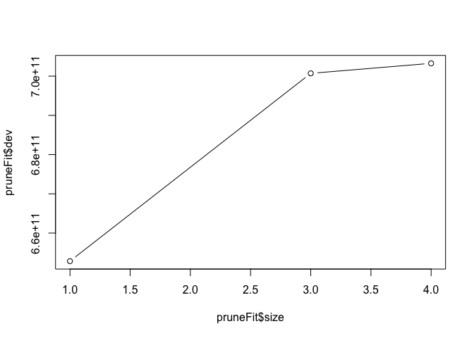
The first model fit to the data will be a regression tree. We’ll use leave-one-out cross-validation to determine the optimal size of the model, as defined by number of splits. By plotting the fitted tree, we can see the deviance by tree size (larger deviance means a better fit).
treeFit <- tree(shares ~ ., data = newsTrain)
summary(treeFit)
##
## Regression tree:
## tree(formula = shares ~ ., data = newsTrain)
## Variables actually used in tree construction:
## [1] "kw_avg_min"            "kw_min_avg"            "min_negative_polarity"
## Number of terminal nodes:  4
## Residual mean deviance:  245100000 = 4.891e+11 / 1996
## Distribution of residuals:
##      Min.   1st Qu.    Median      Mean   3rd Qu.      Max.
## -160500.0   -2326.0   -1839.0       0.0    -539.3  528800.0
pruneFit <- cv.tree(treeFit,
                  K=nrow(newsTrain)-1
                  )


pruneFitFinal <- prune.tree(treeFit, best = pruneFit$size[1])

plot(pruneFit$size ,pruneFit$dev ,type="b")
Boosted tree model
Next, we’ll fit a boosted regression tree. The boosted tree algorithm has a few hyperparameters, and we’ll use repeated 10-fold cross-validation to determine the optimal hyperparameter values. The hyperparameters of the optimal boosted tree is printed below, as well a summary of each fitted model.
fitControl <- trainControl(## 10-fold CV
                           method = "repeatedcv",
                           number = 10,
                           ## repeated ten times
                           repeats = 5
                           )

boostedFit <- train(shares ~ ., data = newsTrain,
                 method = "gbm",
                 trControl = fitControl,
                 verbose = FALSE
                 )

boostedFit$bestTune
##   n.trees interaction.depth shrinkage n.minobsinnode
## 1      50                 1       0.1             10
boostedFit$results
##   shrinkage interaction.depth n.minobsinnode n.trees     RMSE   Rsquared      MAE   RMSESD RsquaredSD    MAESD
## 1       0.1                 1             10      50 12934.69 0.01657501 3928.494 12483.75 0.03507784 1041.924
## 4       0.1                 2             10      50 13118.17 0.01809484 3980.116 12328.95 0.02680138 1029.512
## 7       0.1                 3             10      50 13050.81 0.02427935 4011.278 12367.78 0.03613895 1036.511
## 2       0.1                 1             10     100 13095.39 0.01429058 3990.731 12404.41 0.03006098 1041.272
## 5       0.1                 2             10     100 13281.27 0.01764274 4085.441 12299.41 0.02333652 1049.882
## 8       0.1                 3             10     100 13262.21 0.01696909 4149.086 12351.84 0.02635892 1044.624
## 3       0.1                 1             10     150 13096.10 0.01339196 3984.889 12404.97 0.02800575 1046.104
## 6       0.1                 2             10     150 13510.93 0.01491678 4180.347 12225.15 0.02096103 1040.676
## 9       0.1                 3             10     150 13461.57 0.01662168 4279.897 12306.35 0.02576599 1054.394
Linear regression model
Next, we’ll fit a multiple linear regression model on train data. Summary of the model is printed below.
linearfit<-lm(shares~.,data=newsTrain)
summary(linearfit)
##
## Call:
## lm(formula = shares ~ ., data = newsTrain)
##
## Residuals:
##    Min     1Q Median     3Q    Max
## -48890  -3525  -1330    884 666033
##
## Coefficients: (2 not defined because of singularities)
##                                 Estimate Std. Error t value Pr(>|t|)
## (Intercept)                   -4.023e+03  5.977e+03  -0.673 0.500999
## n_tokens_title                 1.727e+02  1.972e+02   0.876 0.381143
## n_tokens_content              -1.645e+00  1.480e+00  -1.111 0.266507
## n_unique_tokens               -4.946e+03  1.313e+04  -0.377 0.706450
## n_non_stop_words               5.206e+03  1.103e+04   0.472 0.637032
## n_non_stop_unique_tokens       7.999e+03  1.132e+04   0.707 0.479833
## num_hrefs                     -6.136e+00  4.632e+01  -0.132 0.894615
## num_self_hrefs                 2.072e+02  1.284e+02   1.614 0.106642
## num_imgs                       1.663e+01  6.587e+01   0.253 0.800680
## num_videos                     1.327e+02  9.279e+01   1.431 0.152698
## average_token_length          -2.083e+03  1.608e+03  -1.295 0.195424
## num_keywords                  -1.426e+02  2.610e+02  -0.546 0.584962
## data_channel_is_lifestyle     -8.412e+02  2.835e+03  -0.297 0.766756
## data_channel_is_entertainment -1.367e+03  1.825e+03  -0.749 0.454033
## data_channel_is_bus           -1.185e+02  2.729e+03  -0.043 0.965359
## data_channel_is_socmed        -1.247e+03  2.649e+03  -0.471 0.638026
## data_channel_is_tech           9.283e+02  2.687e+03   0.345 0.729769
## data_channel_is_world          1.736e+03  2.735e+03   0.635 0.525717
## kw_min_min                    -2.697e+01  9.672e+00  -2.788 0.005351 **
## kw_max_min                    -4.747e-01  4.734e-01  -1.003 0.316123
## kw_avg_min                     6.337e+00  3.306e+00   1.917 0.055416 .
## kw_min_max                    -3.225e-03  8.806e-03  -0.366 0.714267
## kw_max_max                    -6.517e-03  3.350e-03  -1.945 0.051897 .
## kw_avg_max                    -6.832e-03  5.872e-03  -1.163 0.244777
## kw_min_avg                    -5.994e-01  5.444e-01  -1.101 0.271034
## kw_max_avg                    -5.496e-01  2.400e-01  -2.289 0.022161 *
## kw_avg_avg                     3.988e+00  1.113e+00   3.583 0.000348 ***
## self_reference_min_shares      1.361e-02  7.271e-02   0.187 0.851488
## self_reference_max_shares      1.767e-03  4.189e-02   0.042 0.966357
## self_reference_avg_sharess    -2.321e-03  9.900e-02  -0.023 0.981300
## LDA_00                         5.745e+03  3.129e+03   1.836 0.066530 .
## LDA_01                         5.695e+02  3.425e+03   0.166 0.867942
## LDA_02                         1.701e+03  3.230e+03   0.527 0.598408
## LDA_03                         1.173e+03  3.313e+03   0.354 0.723399
## LDA_04                                NA         NA      NA       NA
## global_subjectivity            1.774e+03  5.685e+03   0.312 0.755119
## global_sentiment_polarity      1.078e+03  1.191e+04   0.091 0.927865
## global_rate_positive_words    -8.026e+03  4.913e+04  -0.163 0.870257
## global_rate_negative_words     8.333e+03  9.036e+04   0.092 0.926531
## rate_positive_words           -1.742e+02  6.982e+03  -0.025 0.980101
## rate_negative_words                   NA         NA      NA       NA
## avg_positive_polarity          5.169e+03  9.397e+03   0.550 0.582314
## min_positive_polarity         -7.749e+03  7.855e+03  -0.986 0.324046
## max_positive_polarity         -3.815e+02  2.934e+03  -0.130 0.896538
## avg_negative_polarity          4.712e+03  8.498e+03   0.555 0.579293
## min_negative_polarity         -5.967e+03  3.072e+03  -1.942 0.052251 .
## max_negative_polarity         -5.085e+03  7.413e+03  -0.686 0.492835
## title_subjectivity            -1.029e+03  1.859e+03  -0.554 0.579908
## title_sentiment_polarity       8.569e+02  1.814e+03   0.472 0.636764
## abs_title_subjectivity         1.423e+03  2.535e+03   0.561 0.574759
## abs_title_sentiment_polarity   6.494e+02  2.735e+03   0.237 0.812344
## ---
## Signif. codes:  0 '***' 0.001 '**' 0.01 '*' 0.05 '.' 0.1 ' ' 1
##
## Residual standard error: 17530 on 1951 degrees of freedom
## Multiple R-squared:  0.03991,    Adjusted R-squared:  0.01628
## F-statistic: 1.689 on 48 and 1951 DF,  p-value: 0.002343
Model Evaluations
Finally, we’ll evaluate the performance of each model by seeking the lowest root mean squared error of its predictions on the test dataset when compared to the actual values in the dataset. This should be a good approximation of the model’s performance on unseen data.
Regression Tree
Below is the RMSE of the optimal (non-ensemble) regression tree:
treePred <- predict(pruneFitFinal, newdata = dplyr::select(newsTest, -shares))
sqrt(mean((treePred-newsTest$shares)^2))
## [1] 15593.79
Boosted Trees
Below is the RMSE of the optimal boosted regression tree:
boostedTreePred <- predict(boostedFit, newdata = dplyr::select(newsTest, -shares))
sqrt(mean((boostedTreePred-newsTest$shares)^2))
## [1] 13551.85
linear regression
Below is the RMSE of the multiple linear model:
linearPred<-predict(linearfit, newdata=dplyr::select(newsTest, -shares))
sqrt(mean((linearPred-newsTest$shares)^2))
## [1] 13401.45