Guide for Using the NHL API

Matt Kasle 9/16/2020

Required Packages

This vignette requires the Tidyverse, httr, and jsonlite packages.

API Helper Function

The NHL provides APIs to access an array of team and player statistics. This vignette provides functions to help users access this data and return well-formatted dataframes for various endpoints. The code below creates a wrapper function for “one-stop-shop” access to a number of endpoints in these APIs.

You can query either API using the function getNHLData(), which takes an available NHL API endpoint, and optionally a team and season, and returns a filtered dataset. You can provide either the team id or the team name.

The available endpoints that a user can provide are:

Records API:

franchises
franchise-team-totals
franchise-season-records
franchise-goalie-records
franchise-skater-records

Stats API:

teams
team.roster
person.names
team.schedule.next
team.schedule.previous
team.stats
statsSingleSeasonPlayoffs

Examples:

knitr::kable(head(getNHLData("franchises")))

id	firstSeasonId	lastSeasonId	mostRecentTeamId	teamCommonName	teamPlaceName
1	19171918	NA	8	Canadiens	Montréal
2	19171918	19171918	41	Wanderers	Montreal
3	19171918	19341935	45	Eagles	St. Louis
4	19191920	19241925	37	Tigers	Hamilton
5	19171918	NA	10	Maple Leafs	Toronto
6	19241925	NA	6	Bruins	Boston

knitr::kable(head(getNHLData("franchise-team-totals", 6)))

id	activeFranchise	firstSeasonId	franchiseId	gameTypeId	gamesPlayed	goalsAgainst	goalsFor	homeLosses	homeOvertimeLosses	homeTies	homeWins	lastSeasonId	losses	overtimeLosses	penaltyMinutes	pointPctg	points	roadLosses	roadOvertimeLosses	roadTies	roadWins	shootoutLosses	shootoutWins	shutouts	teamId	teamName	ties	triCode	wins
11	1	19241925	6	2	6570	19001	20944	953	89	376	1867	NA	2387	184	88037	0.5625	7391	1434	95	415	1341	80	64	500	6	Boston Bruins	791	BOS	3208
12	1	19241925	6	3	664	1875	1923	149	2	3	191	NA	332	0	10505	0.0301	40	183	2	3	135	0	0	49	6	Boston Bruins	6	BOS	326

knitr::kable(getNHLData("team.roster", "Bruins"))

jerseyNumber	person.id	person.fullName	person.link	position.code	position.name	position.type	position.abbreviation
86	8476191	Kevan Miller	/api/v1/people/8476191	D	Defenseman	Defenseman	D
33	8465009	Zdeno Chara	/api/v1/people/8465009	D	Defenseman	Defenseman	D
37	8470638	Patrice Bergeron	/api/v1/people/8470638	C	Center	Forward	C
41	8470860	Jaroslav Halak	/api/v1/people/8470860	G	Goalie	Goalie	G
46	8471276	David Krejci	/api/v1/people/8471276	C	Center	Forward	C
40	8471695	Tuukka Rask	/api/v1/people/8471695	G	Goalie	Goalie	G
63	8473419	Brad Marchand	/api/v1/people/8473419	L	Left Wing	Forward	LW
27	8475186	John Moore	/api/v1/people/8475186	D	Defenseman	Defenseman	D
13	8475745	Charlie Coyle	/api/v1/people/8475745	C	Center	Forward	C
14	8475780	Chris Wagner	/api/v1/people/8475780	R	Right Wing	Forward	RW
20	8475807	Joakim Nordstrom	/api/v1/people/8475807	C	Center	Forward	C
52	8476374	Sean Kuraly	/api/v1/people/8476374	C	Center	Forward	C
35	8476509	Maxime Lagace	/api/v1/people/8476509	G	Goalie	Goalie	G
47	8476792	Torey Krug	/api/v1/people/8476792	D	Defenseman	Defenseman	D
48	8476891	Matt Grzelcyk	/api/v1/people/8476891	D	Defenseman	Defenseman	D
75	8477365	Connor Clifton	/api/v1/people/8477365	D	Defenseman	Defenseman	D
21	8477941	Nick Ritchie	/api/v1/people/8477941	L	Left Wing	Forward	LW
88	8477956	David Pastrnak	/api/v1/people/8477956	R	Right Wing	Forward	RW
10	8478075	Anders Bjork	/api/v1/people/8478075	L	Left Wing	Forward	LW
28	8478131	Ondrej Kase	/api/v1/people/8478131	R	Right Wing	Forward	RW
67	8478415	Jakub Zboril	/api/v1/people/8478415	D	Defenseman	Defenseman	D
80	8478435	Dan Vladar	/api/v1/people/8478435	G	Goalie	Goalie	G
25	8478443	Brandon Carlo	/api/v1/people/8478443	D	Defenseman	Defenseman	D
79	8478468	Jeremy Lauzon	/api/v1/people/8478468	D	Defenseman	Defenseman	D
19	8478485	Zach Senyshyn	/api/v1/people/8478485	R	Right Wing	Forward	RW
74	8478498	Jake DeBrusk	/api/v1/people/8478498	L	Left Wing	Forward	LW
73	8479325	Charlie McAvoy	/api/v1/people/8479325	D	Defenseman	Defenseman	D
82	8479365	Trent Frederic	/api/v1/people/8479365	C	Center	Forward	C
58	8480001	Urho Vaakanainen	/api/v1/people/8480001	D	Defenseman	Defenseman	D
68	8480021	Jack Studnicka	/api/v1/people/8480021	C	Center	Forward	C
83	8480901	Karson Kuhlman	/api/v1/people/8480901	C	Center	Forward	C
26	8480944	Par Lindholm	/api/v1/people/8480944	C	Center	Forward	C

Data Exploration

We’ll explore this data set in a few different ways. Through this process, I’ll demonstrate how to use this set of functions.

First, we’ll read in franchise team totals, filtered to only regular season games and active franchises

# regular season totals for active teams
regularSeasonTotals <- getNHLData("franchise-team-totals") %>% filter(gameTypeId == 2)  %>%  filter(activeFranchise == 1) 

Next, we’ll create some new variables. We’ll create win percentage, goal differential, and home/road win percentage:

regularSeasonTotals$WinPrct <- regularSeasonTotals$wins / (regularSeasonTotals$wins + regularSeasonTotals$losses)

regularSeasonTotals$goaldiff <- regularSeasonTotals$goalsFor - regularSeasonTotals$goalsAgainst

regularSeasonTotals$homeWinPrct <- regularSeasonTotals$homeWins / (regularSeasonTotals$homeWins + regularSeasonTotals$homeLosses)

regularSeasonTotals$roadWinPrct <- regularSeasonTotals$roadWins / (regularSeasonTotals$roadWins + regularSeasonTotals$roadLosses)

Next, we’ll get team data from the Stats API, which has more details about each franchise like division, conference, and time zone, and join that to the previous data set.

# only for active teams
activeTeams <- getNHLData("teams")

# gets division name, venue, other interesting information
activeTeamStats <- dplyr::inner_join(regularSeasonTotals, activeTeams, by = c("franchiseId" = "id")) 

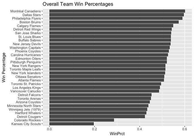
Now, we can plot the all-time win percentage for each team in the league:

g <- ggplot(data = activeTeamStats, aes(reorder(teamName.x, WinPrct), WinPrct))
g + geom_bar(stat="Identity") + 
  labs(x = "") +
  coord_flip() + 
  labs(x = "Win Percentage") +
  ggtitle("Overall Team Win Percentages")

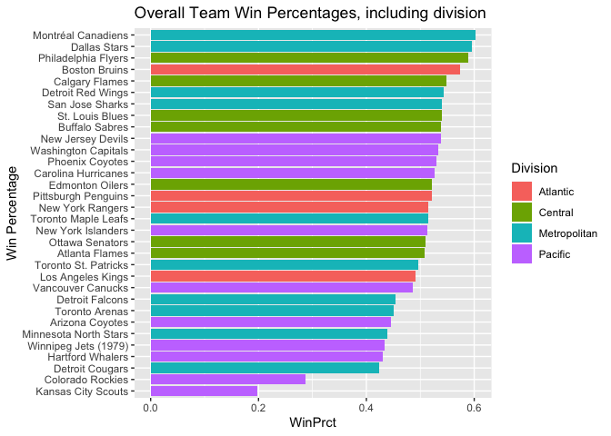
We can also see where teams are located geographically. 12 of the 14 Eastern Conference teams are on the East Coast. By comparison, Western Conference teams are spread out geographically, with teams in central, mountain, pacific, and vancouver time zones.

knitr::kable(table(activeTeamStats$venue.timeZone.id, activeTeamStats$conference.name),
             caption="Team Time Zones by Conference")

	Eastern	Western
America/Chicago	0	5
America/Denver	0	3
America/Detroit	1	0
America/Edmonton	0	1
America/Los_Angeles	0	6
America/New_York	12	0
America/Toronto	1	0
America/Vancouver	0	3

Team Time Zones by Conference

There are four divisions. The Metropolitan division has team closest together by time zone, as all ten teams are on the east coast.

knitr::kable(table(activeTeamStats$venue.timeZone.id, activeTeamStats$division.name),
             caption="Team Time Zones by Conference")

	Atlantic	Central	Metropolitan	Pacific
America/Chicago	0	5	0	0
America/Denver	0	2	0	1
America/Detroit	1	0	0	0
America/Edmonton	0	0	0	1
America/Los_Angeles	0	0	0	6
America/New_York	2	0	10	0
America/Toronto	1	0	0	0
America/Vancouver	0	0	0	3

Team Time Zones by Conference

Now, let’s view all-time win percentages of teams by division:

g <- ggplot(data = activeTeamStats, aes(reorder(teamName.x, WinPrct), WinPrct))
g + geom_bar(stat="Identity", aes(fill=division.name)) + 
  labs(x = "") +
  coord_flip() + 
  labs(x = "Win Percentage", fill="Division") +
  ggtitle("Overall Team Win Percentages, including division")

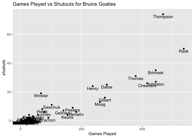
Now let’s explore the team history of a single team. Being from Boston, I will choose my hometown Bruins. We see below that Rask played the most games as the Bruins goalie, but Thompson had by far the most shutouts despite playing about 50 fewer games.

bruinsGoalies <- getNHLData("franchise-goalie-records", team = "Bruins")


g <- ggplot(bruinsGoalies, aes(x = gamesPlayed, y = shutouts))
g + geom_point() +
    labs(x = "Games Played", fill="Shutouts") +
    geom_text(aes(label=lastName),hjust=0.5, vjust=1.2) +
    ggtitle("Games Played vs Shutouts for Bruins Goalies")

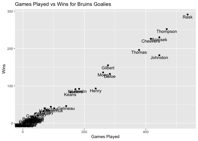
There aren’t many major outliers for wins compared to total games played for Bruins goalies, though Johnston seems to have a much lower win percentage than other goalies. Thompson does not seem to have a much higher win percentage than other goalies, despite the fact that he had the most shutouts.

g <- ggplot(bruinsGoalies, aes(x = gamesPlayed, y = wins))
g + geom_point() +
    geom_text(aes(label=lastName),hjust=0.5, vjust=1.2) +
    labs(x = "Games Played", y="Wins") +
    ggtitle("Games Played vs Wins for Bruins Goalies")

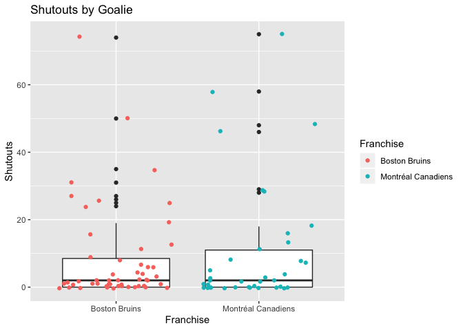
Let’s compare historical goalie performance between the Bruins and their rivals, the Canadiens.

canadiansGoalies <- getNHLData("franchise-goalie-records", team = "Canadiens")
canadianAndBruinGoalies <- dplyr::bind_rows(bruinsGoalies, canadiansGoalies)

g <- ggplot(canadianAndBruinGoalies, aes(x = franchiseName, y = shutouts))
g + geom_boxplot() +
    geom_jitter(mapping = aes(color = franchiseName)) + 
    labs(x = "Franchise", color = "Franchise", y = "Shutouts") +
    ggtitle("Shutouts by Goalie")

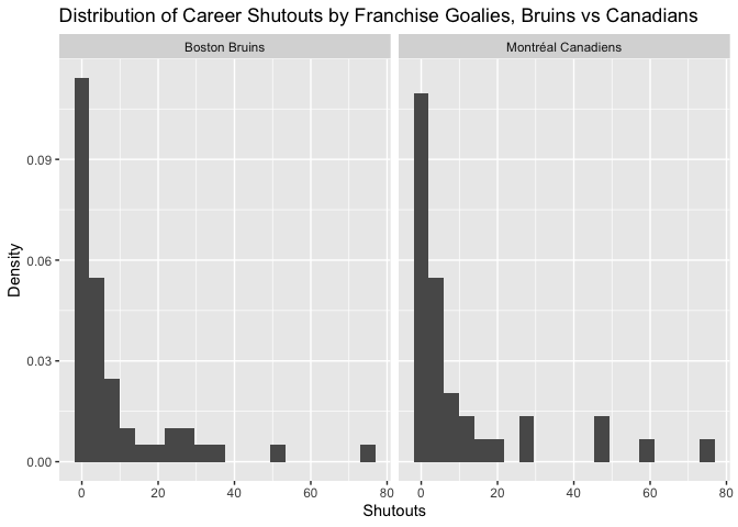
Here is a look at the distribution of the chart above. They look fairly similar.

g <- ggplot(canadianAndBruinGoalies, aes(x = shutouts))
g + geom_histogram(aes(y = ..density..), bins=20) +
    facet_wrap(~ franchiseName) +
    labs(x = "Shutouts", y = "Density") +
    ggtitle("Distribution of Career Shutouts by Franchise Goalies, Bruins vs Canadians")

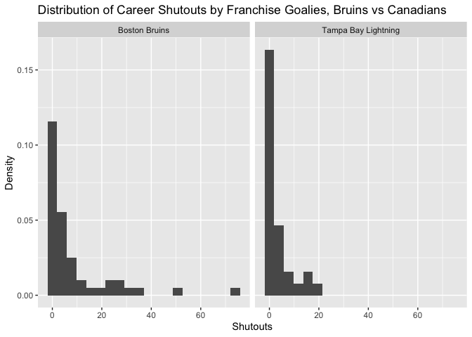
Now, we’ll compare the same distribution with a much newer franchise, the Tampa Bay Lightning. We see that the Lightning have no goalies with more than 25 career shutouts, while the Bruins have multiple goalies with that distinction.

lightningGoalies <- getNHLData("franchise-goalie-records", team = "Lightning")
lightningAndBruinGoalies <- dplyr::bind_rows(bruinsGoalies, lightningGoalies)

g <- ggplot(lightningAndBruinGoalies, aes(x = shutouts))
g + geom_histogram(aes(y = ..density..), bins=20) +
    facet_wrap(~ franchiseName) +
    labs(x = "Shutouts", y = "Density") +
    ggtitle("Distribution of Career Shutouts by Franchise Goalies, Bruins vs Canadians")

We can also look at the performance of teams by their goal differential (how many more or less goals they’ve scored compared to their opponent).

We look at that by division:

knitr::kable(activeTeamStats %>% group_by(division.name) %>% summarise("Avg. Goal Differetial Per Season" = mean(goaldiff,na.rm=TRUE)))

division.name	Avg. Goal Differetial Per Season
Atlantic	262.0000
Central	354.4286
Metropolitan	377.2000
Pacific	-328.5455

We can see by team the most goals that they have allowed.

allGoalies <- getNHLData("franchise-goalie-records")
knitr::kable(allGoalies %>% group_by(franchiseName) %>% summarise("Most Goals Allowed in a Game" = max(mostGoalsAgainstOneGame)))

franchiseName	Most Goals Allowed in a Game
Anaheim Ducks	8
Arizona Coyotes	15
Boston Bruins	13
Brooklyn Americans	10
Buffalo Sabres	11
Calgary Flames	11
Carolina Hurricanes	11
Chicago Blackhawks	12
Cleveland Barons	11
Colorado Avalanche	12
Columbus Blue Jackets	8
Dallas Stars	10
Detroit Red Wings	11
Edmonton Oilers	9
Florida Panthers	8
Hamilton Tigers	16
Los Angeles Kings	11
Minnesota Wild	8
Montréal Canadiens	11
Montreal Maroons	8
Montreal Wanderers	11
Nashville Predators	8
New Jersey Devils	10
New York Islanders	11
New York Rangers	15
Ottawa Senators	11
Philadelphia Flyers	11
Philadelphia Quakers	10
Pittsburgh Penguins	13
San Jose Sharks	11
St. Louis Blues	10
St. Louis Eagles	11
Tampa Bay Lightning	10
Toronto Maple Leafs	13
Vancouver Canucks	13
Vegas Golden Knights	7
Washington Capitals	11
Winnipeg Jets	9

Finally, we’ll summerize home and road performance

# function creates a summary table subsetted on an iris specialties provided by the user
createSummaryTable <- function(division, columns){
  
  # filter dataset by species
  activeTeamsSubset <- activeTeamStats %>% filter(division.name == division) %>% select(columns)
  
  # create summary table
  division_summary <- rbind(apply(activeTeamsSubset,2, min, na.rm=TRUE), 
           apply(activeTeamsSubset,2, quantile, probs=c(.25), na.rm=TRUE),
           apply(activeTeamsSubset,2, median, na.rm=TRUE),
           apply(activeTeamsSubset,2, mean, na.rm=TRUE),
           apply(activeTeamsSubset,2, quantile, probs=c(.75), na.rm=TRUE),
           apply(activeTeamsSubset,2, max, na.rm=TRUE))
  
  division_summary <- round(division_summary, 1)
  # rename index
  rownames(division_summary) <- c("Min.",
                 "1st Qu.",
                 "Median",
                 "Mean",
                 "3rd Qu.",
                 "Max.")
  
  division_summary <- knitr::kable(division_summary, caption = paste("Summary of Division Road Records: ", division))
  return(division_summary)
}

createSummaryTable("Atlantic", c("roadWins", "roadLosses", "roadOvertimeLosses"))

	roadWins	roadLosses	roadOvertimeLosses
Min.	715.0	1039.0	74.0
1st Qu.	741.2	1039.0	86.0
Median	1003.0	1236.5	91.0
Mean	1015.5	1268.2	87.8
3rd Qu.	1277.2	1465.8	92.8
Max.	1341.0	1561.0	95.0

Summary of Division Road Records: Atlantic

createSummaryTable("Pacific", c("roadWins", "roadLosses", "roadOvertimeLosses"))

	roadWins	roadLosses	roadOvertimeLosses
Min.	7.0	66.0	28.0
1st Qu.	142.5	231.5	65.5
Median	275.0	393.0	78.0
Mean	354.5	477.4	69.9
3rd Qu.	644.0	757.0	79.0
Max.	722.0	993.0	94.0

Summary of Division Road Records: Pacific

createSummaryTable("Metropolitan", c("roadWins", "roadLosses", "roadOvertimeLosses"))

	roadWins	roadLosses	roadOvertimeLosses
Min.	3.0	17.0	73.0
1st Qu.	30.8	52.2	75.0
Median	376.0	455.0	76.0
Mean	503.0	616.4	77.6
3rd Qu.	977.2	1203.0	79.0
Max.	1424.0	1607.0	85.0

Summary of Division Road Records: Metropolitan

NHL-API-Vignette

A vignette for the NHL API - project #1 for ST 558 Data Science for Statisticians at NCSU

Guide for Using the NHL API

Required Packages

API Helper Function

Data Exploration